Domain Decomposition Methods

Introduction

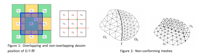
Domain Decomposition (DD) methods represent a class of ad-vanced numerical techniques for solving partial differential equations (PDEs), based on the physical partitioning of a global domain Ω into smaller subdo-mains [1]. This approach addresses computational complexity by distributing the processing load across parallel architectures, reconstructing the global solu-tion through the coordination of local solutions. From a methodological standpoint, a fundamental distinction is made be- tween overlapping approaches, where consistency is achieved iteratively through data exchange across artificial internal boundaries [1], and non-overlapping approaches, which operate by solving interface problems, as seen in Schur com- plement or FETI (Finite Element Tearing and Interconnecting) methods. In literature, the Schur complement method is classified as a ”Primal” approach
(displacement-based), whereas the FETI method represents its ”Dual” coun-terpart (force-based) [3].
Interface management varies significantly depending on the nature of the discretization: while conforming meshes ensure matching nodes at the interface, non-conforming meshes require the use of mortar elements. The latter enforce solution continuity in a weak sense, guaranteeing the optimality of the global approximation while allowing flexible coupling between heterogeneous meshes [2]. A critical advantage of DD methods is their flexibility in local optimiza-tion.
They allow the adoption of different numerical techniques, solvers, or specific mesh refinements within subdomains characterized by geometric singu-larities or high
gradients. This modularity prevents the computational cost of refinement from propagating throughout the entire domain, enabling the use of specialized constitutive laws or integration

Goal

In non-overlapping methods, computational efficiency is achieved by transitioning to a condensed system at the interface. This operation, known as the Schur complement method, involves eliminating the internal degrees of freedom (DoFs) for each subdomain. The resulting system is described by the equation:

Σ h u Γ = χΓ (1)
where Σ h is the subdomain Schur operator (or matrix), representing the con-densed stiffness at the interface, u Γ represents the vector of degrees of freedom
(displacements or unknown values) on the interface boundary Γ and χΓ rep-resents the reaction forces (interface stresses) required to ensure mechanical equilibrium
between subdomains [3].
In industrial contexts, the interface-condensed system is typically solved us-ing iterative Krylov subspace methods, such as the Preconditioned Conjugate Gradient
(PCG), where the DD methods themselves serve as effective precon-ditioners [3]. Once the vector of degrees of freedom on the interface (i.e., the trace of the
solution) is obtained, the global solution can be reconstructed by independently computing it within each subdomain [2]. Furthermore, this modularity allows each
local solver to autonomously adopt its own resolution method, precondi-tioner, or convergence criteria, thereby optimizing the computation according to the specific
characteristics of each region [1]. This work focuses on implementing Domain Decomposition Methods via open-source finite element software, which is particularly well-suited for this type of strategy.

References

[1] Cai, X. (2003). Overlapping domain decomposition methods. In Advanced Topics in Computational Partial Differential Equations: Numerical Meth-ods and Diffpack Programming (pp. 57-95). Berlin, Heidelberg: Springer Berlin Heidelberg.
[2] Ben Belgacem, F., & Maday, Y. (1997). The mortar element method for three dimensional finite elements. ESAIM: Mod´elisation math´ematique et analyse num´erique, 31(2), 289-302.
[3] Gosselet, P., & Rey, C. (2006). Non-overlapping domain decomposition methods in structural mechanics. Archives of computational methods in engineering, 13(4), 515.